The Perpendicular Distance Calculator is a platform-independent Java application that implements a powerful suite of spherical functions for processing observations made during standard line transect surveys. Line transect sampling a commonly used distance sampling method that can be used for estimating the density and/or abundance of biological populations.

Visit our main page to learn more about the Center for Biodiversity and Conservation.

Download

Platform independent jar | PerpendicularDistanceCalculator_v1.2.2.zip (32.7 KB)
Source code | https://github.com/persts/GeographicDistanceTools

Citation

If you wish to cite the background or documentation we suggest the following format:

Ersts,P.J., Horning, N., and M. Polin[Internet] Perpendicular Distance Calculator(version 1.2.2) Documentation. American Museum of Natural History, Center for Biodiversity and Conservation. Available from http://biodiversityinformatics.amnh.org/open_source/pdc. Accessed on .

If you use the application on data that results in a publication, report, or online analysis, we ask that you include the following reference:

Ersts,P.J.[Internet] Perpendicular Distance Calculator(version 1.2.2). American Museum of Natural History, Center for Biodiversity and Conservation. Available from http://biodiversityinformatics.amnh.org/open_source/pdc. Accessed on .

Background and Documentation

Peter J. Ersts*, Ned Horning*, and Marco Polin**

Introduction

Line transect distance sampling is a suite of related methods commonly used for estimating the density and/or abundance of biological populations (Buckland et al. 2001). Of these methods, line transect distance sampling is the most broadly applied technique. The general concept behind line transect surveys, as summarized in Thomas et al. (2002), involves an observer or team of observers traversing a linear search path (i.e., transect or transect leg) looking for objects of interest. Objects of interest can be either a single animal or plant, or groups of animals or plants. For each object of interest detected, observers record the perpendicular distance from the object of interest or center of group to the transect leg. Perpendicular distances are used to model detection functions that estimate the proportion of objects present but undetected during the survey process. Detection functions are a pivotal component in calculating reliable estimates of population abundance and/or densities. Detailed, in-depth descriptions of distance sampling methods can be found in Buckland et al. (2001, 2004).

Under ideal conditions, observers can directly measure perpendicular distance using a tape measure or more advanced equipment, such as, a laser range finder. However, for perpendicular distances exceeding 1000 meters or surveys for highly mobile, inconspicuous or easily displaced animals, it may not be possible to directly measure perpendicular distance; in which case it is also necessary to evaluate if this sampling method is appropriate to begin with. Alternatives to direct measurement involve the derivation of perpendicular distance from measurements taken at the time of initial detection. These measurements become inputs to standard trigonometric or geodesic equations.

The most widely implemented method for deriving perpendicular distance is founded in planar geometry and simply involves solving for one side of a right-angled triangle. This planar method only requires two inputs, a radial distance, which we will call a detection distance, and an angle. The detection distance is the distance from the observers to the object of interest at the time of initial detection. The angle is traditionally defined as the angle between the transect leg and a line connecting the observers and the object of interest, or center of group, at the initial time of observation. While the planar method is intuitive and easy to implement, this method requires an angle to be measure relative to the transect and does not directly provide any geographically explicit information regarding the objects of interest. As GPS receivers become common pieces of equipment in researchers' inventories, other alternatives to the planar method for calculating perpendicular distance are possible. We describe a robust, alternative method for calculating perpendicular distance that implements spherical geometry.

Methods

The following methods implement basic vector, geometric and trigonometric procedures, which form the basis for all geodetic (e.g., Bomford 1971), celestial (e.g., Green 1985, Danby 1988) and navigational (e.g., Bowditch, 1995) calculations. Various implementations and discussions of the equations that follow can also be found on numerous Internet resources (e.g., Ed Williams's Aviation Formulary, The Math Forum at Drexel University).

For this discussion, all angles and geographic coordinates are expressed in radians, unless otherwise noted. Several of the following geodesic equations require modulus and arctangent operations. The modulus or MOD function returns the remainder when one number is divided by another. For example, 22 / 7 = 3 remainder 1, thus 22 MOD 7, or MOD(22, 7) as it may appear in a programming language or spreadsheet application, would return 1. Likewise, 2 MOD 7 would return 2 because 2 / 7 = 0 remainder 2. Many spreadsheet applications and programming languages have several arctangent functions. The arctangent operation implemented in the following methods, typically called atan2, uses the signs of the two input variables to determine the quadrant of the result. Additionally, to fully understand the methods that follow, a general understanding of basic vector mathematics is required.

Planar method

To calculate perpendicular distances (Δpd) using planar geometry, the observers are required to record a detection (radial) distance distance (D) and a angle (Θooi) relative to the transect leg.

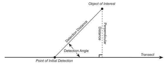
The perpendicular distance can simply be expressed as one side of a right-angled triangle,

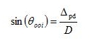
which can be rewritten as,

The resulting perpendicular distance will be in the same units as the detection distance. While this planar approach for calculating perpendicular distance is simple and intuitive, this method requires that angles relative to the transect leg be recorded at the time of initial detection. A common method for determining the angle is through the use of an angle board. Angle boards are easy to implement and construct but hastily or poorly constructed angle boards can be very imprecise. Without the use of specialized equipment, which may be prohibitively expensive or require careful calibration and large, stable working platforms, it can be difficult or even impossible under many field conditions for observers to accurately record the angle relative to the transect leg. Furthermore, angle boards are generally fixed to the survey platform. Therefore, an angle board often provides an angle and subsequent perpendicular distance relative to the orientation or midline of survey platform rather than the transect leg itself. Thus, navigational error and movement of the survey platform (e.g., a boat on rough water) may cause the midline of the survey platform to deviate from the transect, impacting the accuracy and validity of the angle measurement.

Spherical approach

The spherical approach for deriving perpendicular distances is accomplished by determining the intersection of two great circles.

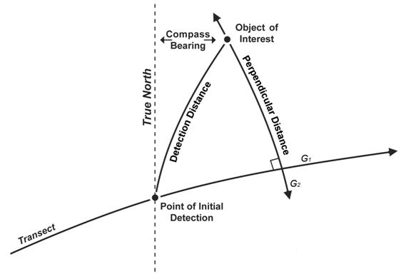
A great circle is a circle that is produced by the intersection of the Earth's surface with a plane passing through the center of the Earth. The shortest distance between two points on the Earth's surface is an arc or segment of a great circle. The first great circle (G1) referenced by this method is the great circle passing through the start and end point of the transect leg. The second great circle (G2) intersects G1 at a 90 degree angle and passes through the geographic location of a sighting or object of interest. The perpendicular distance is the shortest arc length between the object of interest and the intersection of G1 and G2.

In this method, the angle is just a compass bearing. Thus, the angle is not relative to the transect leg nor the survey platform but instead represents the angle east of True North. The benefits of this spherical approach to calculating perpendicular distance are 1) the result is "geometrically" correct, 2) coordinate data are derived for each object of interest, and 3) the resulting perpendicular distance is not affected by navigational error or orientation of the survey platform. This spherical approach assumes that 1) the Earth is a perfect sphere, 2) the observers or survey platform implement great circle navigation rather than rhumb line navigation (simply following a course of constant bearing), and 3) the observers correct their compass for magnetic declination and magnetic signature of the survey platform. The geographic coordinates of the object of interest are derived post survey from the geographic coordinates of the observers or survey platform at the time of initial detection (Latobs and Lonobs), the detection distance (D), and the bearing to the object of interest (θooi) using following equations;

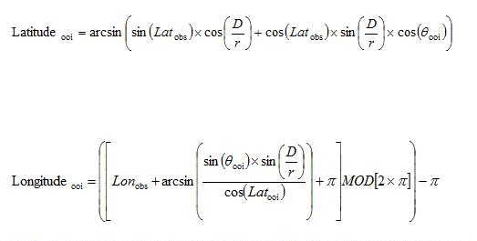
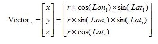
where r is the radius of the spherical representation of the Earth. It is important to note that D and r must be in the same units of measurement and the calculation of Longitudeooi utilizes derived Latitudeooi not Latitudeobs. The initial step in calculating perpendicular distance using spherical geometry is to transform the geographic coordinate system into a three dimensional Cartesian coordinate system so that each geographic coordinate pair (i.e., latitude and longitude) is represented as a vector with three terms (i.e., x y z). For this transformation, 0 ≤ longitude ≤ 2π and latitude is actually defined as the colatitude (π - latitude) where 0 ≤ colatitude ≤ π. This transformation is applied to the spherical coordinates for the start of the transect leg (Ts), the end of the transect leg (Te) and the derived location of the object of interest (Pooi).

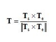
The second step is to cross normalize the vectors representing the start (Ts) and end (Te) of the transect leg, which produces a vector (T) that has unit length and is perpendicular to the great circle (G1) passing through the start and end of the transect leg.

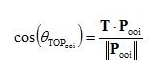
The next step is to calculate the dot product of T and Pooi which will equal the cosine of the angle between vector T, the center or origin of the Earth (O), and the Pooi.

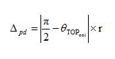
The difference between θTOPooi and π / 2 is the angle subtended by the segment of the great circle (G2) passing through the object of interest (Pooi) and perpendicular to the transect leg, that represents our perpendicular distance. The length of such great-arc segment is the perpendicular distance (δpd) and can be obtained by multiplying by r, the radius of the spherical representation of the Earth. The resulting perpendicular distance will be in the same units as r.

Discussion

Spherical computations are undoubtedly more involved. Therefore, we have developed and released the Perpendicular Distance Calculator, a platform independent, open-source implementation of the approach described above. This spherical approach for calculating perpendicular distance is an alternative method to the planar approach. The greatest advantage of the spherical approach over the planar approach is that the results are not affected by navigational error. An added benefit of this spherical approach is that the actual geographic localities for each object of interest or sightings can easily be derived. Having the coordinates of sightings creates possibilities for other types of spatial analysis and modeling opportunities (e.g., Hedley and Buckland 2004). Furthermore, perpendicular distances can be calculated directly from geographic coordinates (i.e., latitude and longitude) without the need for additional spatial software, which is often expensive and requires extensive specialized knowledge to properly use.

Results obtained using this spherical method will only be as accurate and precise as the measurements used as inputs. High quality sighting compasses allow for readings in half degree increments and, if used properly, represent a significant improvement over handmade angle boards. Detection distances that are estimated by eye will be far less accurate than distances estimated through other means and imprecise distance estimates probably represent the single greatest source of error in distance sampling. In general, inaccurate or imprecise inputs will affect the spherical approach as much as any other method. Furthermore, accuracy of results can also vary between GPS receivers and the numerical precision used through the calculation. For example, assuming that the radius of the Earth is 6378137 meters (WGS 84 definition), one meter at the Equator is equivalent to 0.000008983 degrees. Thus, it is important to maintain as many significant digits as possible during data recording and subsequent calculations.

The assumption that the Earth is a perfect sphere is inaccurate, but the violation of this assumption does not introduce significant adverse effects or biases to the resulting perpendicular distances due the length of distances being calculated and traversed relative to the radius of the Earth; poor detection distance estimates are a far greater source of error. The assumption that observers implement great circle navigation rather than rhumb line navigation requires special attention. As an observer moves along a great circle, the compass bearing to their destination is constantly changing, which makes precise navigation along great circles over long distances by compass impractical. The disparity between the rhumb line and great circle distance becomes more significant as one approaches the poles. Accurate and precise great circle navigation is only possible with the aid of an electronic navigation device. However, with the increased accessibility and popularity of GPS receivers, researchers wishing to implement this spherical methodology will not be limited by the requirement to implement great circle navigation along transect legs

Literature cited

Bomford, G. 1971. Geodesy, Oxford University Press, Ely House, London. UK.

Bowditch, N. 1995. The American Practical Navigator: An Epitome of Navigation 1995 edition, Defense Mapping Agency Hydrographic/Topographic Center, Bethesda, MD, USA.

Buckland, S.T., D. R. Anderson, K. P. Burnham, J. L. Laake, D. L. Borchers, and L. Thomas. 2001. Introduction to Distance Sampling, Oxford University Press, Oxford, UK.

Buckland, S.T., D. R. Anderson, K. P. Burnham, J. L. Laake, D. L. Borchers, and L. Thomas eds. 2004. Advanced Distance Sampling, Oxford University Press, Oxford, UK.

Danby, J. M. 1988. Fundamentals of Celestial Mechanics 2nd ed., rev. ed., Willmann-Bell, Richmond, USA.

Drexel University. 2007 Jan 10. The Math Forum @ Drexel. http://mathforum.org. Accessed 10 Jan 2007.

Green, R. M. 1985. Spherical Astronomy, Cambridge University Press, New York, USA.

Hedley, S. L., and S. T. Buckland. 2004. Spatial models for line transect sampling. Journal of Agriculture, Biological and Environmental Statistics, 9, 181-199.

Thomas, L., S. T. Buckland, K. P. Burnham, D. R. Anderson, J. L. Laake, D. L. Borchers, and S. Strindberg. 2002. Distance Sampling. Pages 544-552 in A.H El-Shaarawi and W.W. Piegorsch eds. Encyclopedia of Environmetrics. John Wiley & Sons, Chichester, UK.

Williams, E. 2007 Jan 10. Aviation Formulary V1.43. http://williams.best.vwh.net/avform.htm. Accessed on 10 Jan 2007.

Acknowledgements

We would like to thank Eleanor Sterling for her unwavering support and dedication to the study and conservation of biodiversity. Liz Nichols, Eugenia Naro-Maciel, Kevin Koy, Matthew Leslie, Samantha Strindberg, and an anonymous reviewer provided valuable comments and suggestions that strengthen the districton of this method. We would also like to thank FFEM, Collectivite Departementale de Mayotte, Observatoire des Mammiferes Marins, Office National de la Chasse et de la Faune Sauvage, Direction de l'Agriculture et de la Foret, l'Association MEGAPTERA, Howard Rosenbaum, and the Captain and crew of the Turquoise for making the survey, for which this application was developed, possible. This work was partially funded by NASA under award No. NNG05G041G and award No. NA055SEC46391002 from the National Oceanic and Atmospheric Administration, U.S. Department of Commerce.

Using the Perpendicular Distance Calculator

On most systems, you should be able to activate the application by double clicking on the JAR file. The application can also be started by opening a terminal window or command prompt and entering

to manually launching the application. PerpendicularDistanceCalculator_v1.2.2.jar requires JRE version 1.5.x or higher. If the application does not load, check your version of java by opening a command prompt or terminal window and typing java -version. You can also just download the newest version of Java from http://java.com

Calculating Perpendicular Distances

Manually calculating perpendicular distances using spherical methods is time consuming and prone to errors. The Perpendicular Distance Calculator greatly simplifies this process with its intuitive, easy to use interface.

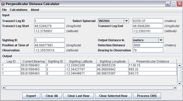
to calculate perpendicular distance using spherical methods you will need the following data:

All fields in the in the Perpendicular Distance Calculator main window must be filled in. Fields in the upper half of the input area pertain to the transect or transect leg. Fields in the lower portion of the input area pertain to data collected at the time of the initial detection. Once all fields are filled in, the calculation can be completed by pressing the [Process OBS] button. Results will appear as rows of the table in the output area. The calculation returns the following data:

You can clear all rows in the output area by clicking the [Clear All] button. You can delete the last row by clicking the [Clear Last Row] button. Alternatively you can delete interior rows by selecting it with your mouse and clicking on the [Clear Selected Row] to remove it. Results can be exported into a tab delineated file by simply clicking the [Export] button. A file dialog will open and as you for a filename.

Examining Navigational Accuracy

You can check the navigational accuracy of the observer of survey platform by entering the geographic coordinates of the observer or survey platform at the time of the intial detection, the geographic coordinates for the start and end of the corresponding transect or transect leg and simply 0 for the Detection Distance and Bearing to Observation. Clicking the [Process OBS] button will calculate the perpendicular distance between the observer or survey platform and the transect, thus indicating the level of navigational accuracy and potential bias associated the corresponding sighting.

Calculating Great Circle Distances

A great circle is a circle that is produced by the intersection of the Earth's surface with a plane passing through the center of the Earth. The shortest distance between two points on the Earth's surface is an arc, which is simply a segment of the great circle passing through said points.

The Perpendicular Distance Calculator provides you with the ability to calculate the distance between to geographic locations. This calculation can be activated by selecting Calculations -> Great Circle Distance from the menu in the main window.

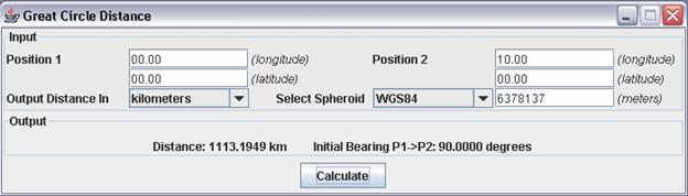
This calculation simply requires the geographic coordinates, in decimal degrees, for two points on the Earth's surface. After selecting your output units and spheroid, press the Calculate button to compute the results. This calculation will return both the distance between your two points but also the initial compass bearing from Position 1 to Position 2. Remember, as you travel along a great circle, your compass bearing to your destination is always changing.

Calculating Intermediate Great Circle Points

In certain circumstances, you may wish to divide a great circle into even intervals. The Intermediate Great Circle Points feature will do just that. You can activate this feature by selecting Calculations -> Intermediate Great Circle Point from the menu in the main window.

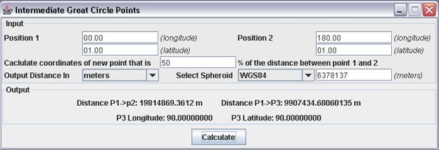
In addition to the geographic coordinates for two points on the Earth's surface, the Intermediate Great Circle Points calculation requires you to enter the percentage of the distance along the great circle, connecting Position 1 and Position 2, at which Position 3 lies. After selecting your output units and spheroid, press the Calculate button to compute the results. This calculation will return the great circle distance between Position 1 and Position 2 great circle distance between Position 1, and Position 3 and the longitude and latitude for Position 3.

This library and software are based upon work partially supported by NASA under award number NAG5-12333. Additionally, this library and application were also prepared under award No. NA04AR4700191 from the National Oceanic and Atmospheric Administration, U.S. Department of Commerce. The statements, findings, conclusions, and recommendations are those of the author(s) and do not necessarily reflect the views of the National Oceanic and Atmospheric Administration or the Department of Commerce.